How to Measure Trading Success

After you have been trading for a certain period of time, recording your trades and creating a performance track record, you're ready to evaluate your results. But how do you define “good trading system” vs. “bad trading system”? And how can you showcase your results, in order to attract capital or investors? Many people simply look at the net profit assuming the system with the more profit must be the better system. It's like a doctor saying “this man looks healthier than the next” without doing a proper tests. In this article, we'll explore some solid metrics to evaluate your trading results that can tell you much more about your trading than the mere profit margin can.

1. Why do we need performance metrics?
Imagine wanting to allocate capital to a trader that has a proven strategy. You have many traders to choose from, that trade many different “systems” they have created. Which one do you choose? There is no one single score you can use that will work for everyone since we all have unique risk tolerances and definitions on what we consider tradable. Likewise, not all scoring systems are equal or perform under all circumstances. However, there are key system performance metrics that you should use during the system development process, and as you progress as a trader, that will show you more information about your trading – typically in a risk-adjusted way.
Large profits accumulated by taking equally or larger risks are not as palatable as slightly smaller profits accumulated by taking small risks. Also, large profits mixed with large losses are less palatable than steady minor P&L swings. This is what we want to measure: how consistent we are at taking on risk that produces equal or larger reward. The metrics that we are going to explore in this article are:
a) Standard Deviation (or “volatility”)
b) Sharpe Ratio
c) Sortino Ratio
d) K-Ratio
Another key performance metric is your system expectation, which we have covered in a previous article.
2. What is Standard Deviation?
Standard deviation is a measure of statistical dispersion. In plain English it's a way of describing how spread out a set of values are around the mean of that data set. For example, if you have a set of trade outcomes (in P&L terms or %R terms), you can easily work out the arithmetic mean (just sum up all the values and then divide by the number of trades). However, knowing the mean (or average, as it's more commonly called), doesn't tell you anything about how orderly the results are. Were all your trades more or less 2R? Did you have 3-4R trades and 1-2R losses? Did you have 10R trades and 10R losses? You can have exactly the same average P&L with very different distribution characteristics. Look at the graph below.
In the graph above, we have 2 sample distributions of hypothetical p/l sets. On the X axis we would be viewing all the $ earned/lost that the trades have experienced, from the largest loss to the largest profit. On the Y axis, we would have the number of trades that had one identical outcome.
What the graph is telling us visually, is that although the two traders have had an equal average performance (mean value), the trader represented with the red p/l distribution has had a much wider spread of returns. He's had larger losses and larger gains than the trader represented with the blue distribution. What we would find is that the standard deviation of the red distribution would be higher than the blue distribution. We would prefer to be trading with a smaller standard deviation around our average return.
How do I calculate it?
The basic idea of the standard deviation is that you're measuring variations around the mean value. Some of those values will be below the mean, some above and sometimes you'll have some that are equal to the mean. In other words some of the differences between the individual measurements will be positive (more than the mean), some will be negative (below the mean) and some will be zero (directly equal to the mean). Now just adding these differences up is useless because the positive and negative values will cancel each other out. For example, to take an incredibly simplistic case: if you've got two trades that gave $100 profit and $50 profit, the mean is equal to ((100+50)/2) = $75. The differences are [(100-75) = 25] and [(50-75) = -25]. Adding these together gives us a total variation of 0. But we know that there's not zero variation around that mean value!
So, to get around this problem each of the variations around the mean is squared. When you square a negative value you get a positive value. So, to work out the standard deviation we square all of the differences from the mean, add them all up, and divide by one less than the number of values in our set. This new number is called the variance. Now we take the square root of the variance (which is reversing the squaring we did earlier so that our number is closer to the original differences), and that's the standard deviation.
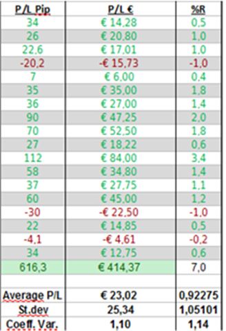
Here's an example of how you can calculate the function (St.Dev or Dev.St on Excel or OpenOffice):
At the bottom I have also added another calculation: the Coefficient of Variation. This measure is the standard deviation divided by the average p/l, and is basically a “noise to signal” ratio. It shows you how good your average p/l can predict your future performance. Values close or inferior to 1 are what you should be aiming for.
What is the fuss about the 'normal distribution' in statistics?
If your p/l set is “normally distributed”, in other words you've got most data near the mean and the further away you get from the mean the fewer measurements you have, then the standard deviation gives you extra information:
·Around 68% of data are within one standard deviation of the mean
·Around 95% of data are within two standard deviations of the mean
·Around 99% of data are within three standard deviations of the mean
So taking the values from above: if the average P/L is 23 and the standard deviation is 25, you can expect to see about 68% of values in the range -2 to 48, and 95% to be in the range -27 to 73. And anything below -27 or above 73 is going to be very rare (Black Swan area).
Confusion between mean absolute deviation and standard deviation
Some charting packages include a “standard deviation” indicator. We should not confuse this measure with the standard deviation we are talking about in this article. To say “the asset moves on average 1% a day in absolute value” is different than saying “the standard deviation of the asset is 1%”. There has been much confusion in the financial industry on this point, and Nassim Taleb has actually written a short essay on this, back in 2007.
If an instrument has a daily standard deviation of 1%, it does not move on average 1% per day. In a “normal distribution”, the ratio of standard deviation to mean absolute deviation is 1.25. So if the mean deviation is 1%, then the standard deviation is 1.25%. If the standard deviation is 1%, the mean deviation is 0.8%. Also, when annualizing the standard deviation of any particular dataset, remember to multiply by the square root of time: so for annualizing a daily standard deviation measure, be sure to multiply by the square root of 365.
Also, the standard deviation of certain instruments will rise/fall in line with the value of the instrument. The standard deviation of Apple or Google will be very different than the standard deviation of EURUSD. So it would be useful to divide the standard deviation by the price of the security in order to get a percentage read that could make comparisons possible through various asset classes.
Finally, standard deviation is also called “volatility” and you will frequently find it cited as ?.
3. Sharpe Ratio
Now that we understand the key concepts of mean (average) and volatility (?), we can proceed to calculate other risk measures that use the same metrics. Close to 50 years ago, W. Sharpe [1966], introduced a measure for the performance of mutual funds and proposed the term “reward-to-variability ratio” to describe it. While the measure has gained considerable popularity, the name has not. The term “Sharpe Ratio” has become the most popular (Morningstar [1993, p. 24]).
The Sharpe Ratio is created as follows:
Rft = return of the trader in period t
Rbt = return on the benchmark in period t, which is frequently the “risk-free” rate of return (like the return available on a government bond)
Such as Dt = Rft - Rbt
Dt = differential return in period t
Then calculate the average value of Dt (which we will call AvgD) over the historic period from t=1 through T, and the standard deviation of Dt (which we call ?D) over the historic period. At this point we can calculate the Sharpe Ratio:
Sharpe Ratio = AvgD / ?D
The ratio indicates the historic average differential return per unit of historic variability of the differential return.
It is a simple matter to compute the Sharpe Ratio using Excel or OpenOffice. The returns of the trader are listed in one column and those of the desired benchmark in the next column. The differences are computed in a third column. Standard functions are then utilized to compute the components of the ratio. For example, if the differential returns were in cells C1 through C10, a formula would provide the Sharpe Ratio using Excel:
AVERAGE(C1:C10)/STDEV(C1:C10)
The higher a trader's Sharpe ratio, the better his returns have been relative to the amount of risk he has taken. Vice versa, the higher a trader's standard deviation, the higher his returns need to be to earn a high Sharpe Ratio. Conversely, traders with lower standard deviations can have a higher Sharpe ratio if they have consistently decent returns. Keep in mind that even though a higher Sharpe ratio indicates a better historical risk-adjusted performance, this doesn't necessarily translate to a lower-volatility trading system. A higher Sharpe ratio just means that the trader's risk/return relationship is more proportional.
It's easier to compare returns of all types using the standard-deviation-based Sharpe ratio than with the beta-based alpha concept (alpha is a measure of how much the investment has outperformed the benchmark due to active management). Unlike beta— the amount of market risk exposure an investment has had, which is usually calculated using different benchmarks for stock and bond funds—standard deviation is calculated the exact same way for any type of performance, be it stock, bond or currency returns. We can therefore use the Sharpe ratio to compare the risk-adjusted returns of stock traders with those of bond traders and currency traders.
As with alpha, the main drawback of the Sharpe ratio is that it is expressed as a raw number—of course, the higher the Sharpe ratio the better—but given no other information, you can't tell whether a Sharpe ratio of 1.5 is good or bad. Only when you compare one trader's Sharpe ratio with that of another trader (or index of traders in the same asset class) do you get a feel for his risk-adjusted return relative to others.
Ideal values for the Sharpe Ratio would be above 1. A ratio of 2 is very good and a ratio of 3 is exceptional.
Another debate regards the correct benchmark to choose when creating the Sharpe ratio. For many investments, the risk-free rate of return might be an ideal choice (i.e., the annual return that you could get on a long term government bond). But for traders, which are active managers, other benchmarks would probably be more adequate. We will talk about benchmarks in a separate article, but ideally when comparing your performance as a trader to a benchmark, the risk-free rate is not as satisfactory as it is for other types of investments.
4. Sortino Ratio
Both the Sortino and the Sharpe ratio were designed to help investors compare returns from different sources. The Sharpe ratio, as we have seen, subtracts the performance of the investment from a benchmark – that in many cases is called the “risk free rate”. Sortino starts by denying the availability of any “risk-free” investment. After all, if there is no risk, there is no reward. His assumption may be open to debate, but his logic can take us a step further along the path of “risk”. After all, the Sharpe ratio “unfairly” penalizes volatility: upside volatility and downside volatility are given the same importance. But to investors, upside volatility is actually good!
Just imagine having to explain your trading records to someone: “yeah, the performance was much more volatile than expected...we had a 5% return in January, a 10% return in February, a 3% return in March, and a 40% return in April...” Not exactly a bad thing to have upside volatility now, is it?
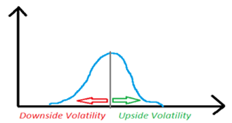
Usually investments have a symmetrical volatility profile.....
Sortino overcomes this, by looking only at the downside deviations – the ones that we do not like. The caveat to this logic is that most (not all) investments have a symmetrical volatility – wild to the upside AND to the downside or calm to the upside AND to the downside.
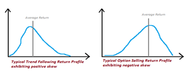
….but certain trading strategies can have the same Sharpe Ratio but different risk profile
For Sortino, “risk” is defined not as the variability of an investment, but as the failure to meet your investment objectives. The definition of “risk” has important consequences for each one of us and there is not a uniform way to define it, so it's also quite instructive to see two different interpretations (Sharpe vs. Sortino) one against the other. In the above graph, the two strategies can have the same Sharpe Ratio, but the positive skew for trend following actually means that the trader is taking on less risk than the Sharpe ratio predicts, while the negative skew of the option selling strategy means that the trader is taking on more risk than the Sharpe ratio predicts.
Just as a side-note, skewness is the degree to which the return distribution is spread around the average return. A trend following strategy that has fewer losses of larger magnitude and frequent winners of smaller magnitude could have a positive skew, meaning that the returns are not equally balanced between profits and losses. In this lies the importance of money management for a trader: you can have a positive skew in your trading, as long as you cut your losses to 1R, and have a wide range of profitable trades that will give you the positive skew characteristic.
So the Sortino ratio is actually a better choice than the Sharpe Ratio, when measuring returns that could have a non-neutral skewness. Here is how it's defined mathematically:
R = average return over the time period selected
T= Target or required rate of return for the strategy, which was initially the Minimum Accepted Return and then changed to the Desired Target Return.
TDD = Target Downside Deviation, which is the root-mean-square of the deviations of the realized return's underperformance from the target return where all returns above the target return are automatically set to 0.
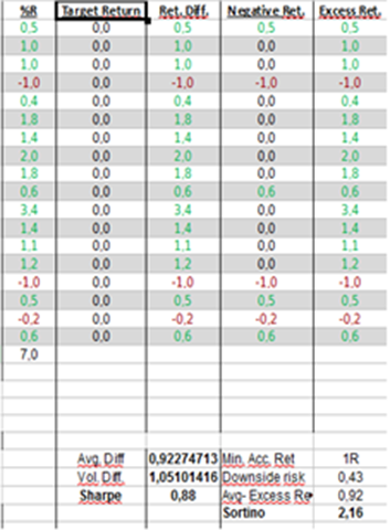
Below we have 2 spreadsheet examples calculating our ratios using %R as the return variable. In the first example, we have imposed a strict 1R minimum target return. In the second example, we have imposed a loose 0R target return (so as long as you're not losing money you're ok). These returns are arbitrary and are not the only example (or the best for that matter) of what can be used as a target return. Also, we are not using annualized % returns here, in an attempt to make the example clear and adequate for trading purposes.
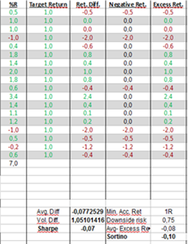
1R target return. We are net profitable, but our ratios look bad.
Zero-R target return. We are net profitable and our ratios are acceptable.
5. K-Ratio
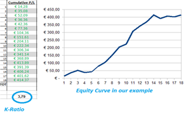
The K-Ratio is completely different than the previous ratios. Like the other metrics, it's a return vs. risk metric, where the numerator is an expression of return and the denominator an expression of risk. The numerator is the slope of the best-fit regression line superimposed over a cumulative return series. The steeper the slope, the faster the growth rate of the account. The denominator is the standard error of that best-fit regression line.
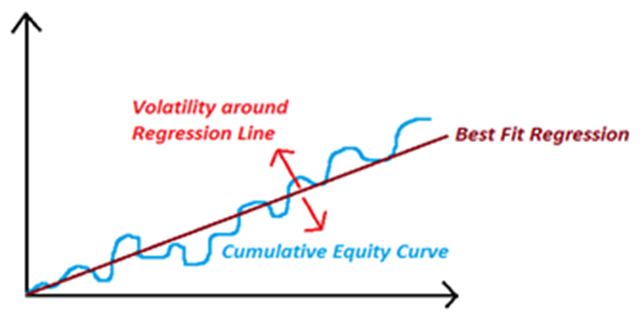
A visual representation of the Best Fit Regression Line
The ratio was invented by Lars Kestner in 1996 in his article “Measuring System Performance” for Stocks & Commodities Magazine. It's an interesting ratio because it's basically a measure of how consistent a trader is performing over time. The ratio should be above zero, which means that you are constantly making progress on your account.
Higher values of the K-Ratio can be obtained by having a small volatility of returns, and a higher hit rate. Having a 70% hit rate, a 1.5R average profit and 1R average loss will be much smoother than a 50% hit rate with a 2R average profit and 1R average loss. The K ratio rewards steady, consistent gains, rather than infrequent, yet huge gains.
Here is how to calculate the K Ratio:
Slope of best fit regression line upon cumulative return line/ standard error of best fit line
which on a spreadsheet means:
Column A = trade number 1,2,3....100
Column B = cumulative equity curve from line 1 to ….100
K-ratio = (SLOPE(column B, Column A)*SQRT(DEVSQ(column A))/(STEYX(column B,Column A)*SQRT(N° Trades))
Kestner, in 2002, upgraded his formula to account for a small error regarding the scale of the K-Ratio.
The 2003 ratio = original K Ratio / Square root of number of observations
To sum up: if you should retain anything at all from this article, retain the fact that if you plan on presenting your trading results to potential investors, or seeking out funding, you will most likely be required to present similar statistics. Investors do not really care about how profitable you are: they care about your risk-adjusted profile. It doesn't take an immense knowledge in statistics to compile a good-looking trading record with some fancy ratios in it, and this article can help you present your records better. The bottom line on all risk-adjusted ratios is this: if you can manage to make steady profits of 1R or more, contain your losses and keep them as close as possible to 1R (or less) and get over a 50% win ratio, then your statistics will automatically be good.

